The Aggregate Expenditure Model Explained (with Graphs)

The Aggregate Expenditure Model comes from Keynesian economics; it is a model that attempts to formulate the complex interactions between the four components of total expenditure i.e., consumption, investment, government spending, and net exports.

Special attention is given, as is usually the case with Keynesians, to consumption. Consumption expenditure is regarded as an endogenous variable in the aggregate expenditure model because it is assumed to be dependent upon disposable income (and thus output), and we can build that into the model. The other three components are regarded as being exogenous variables, and subject to volatility (especially investment spending).

Technically speaking, net exports are also somewhat related to disposable income since spending on imports is directly related to disposable income; only exports are truly exogenous. More advanced treatments of the model do attempt to account for this, but it doesn’t affect the concept and so I will proceed with the standard treatment of assuming net exports to be exogenous.

I should point out that the aggregate expenditure model is closely related to the standard Keynesian consumption function, and readers are well advised to start by reading my article on that as a precursor to this article, because the aggregate expenditure model is really just an extension of the same ideas.

The Aggregate Expenditure Formula

The term aggregate expenditure (AE) is interchangeable with the term aggregate demand (AD), and can be expressed by the simple formula:

AE = C + I + G + (X-M)

If you have read my article about aggregate demand then this formula will look very familiar, the only difference is that it starts with AE rather than AD. The point here is not to rehash the ground already covered in other articles, but to break down in extra detail the key components of the model, explain how they work, and explore the implications for fiscal policy and economic stability.

With that in mind, a further step in the development of the formula above is to incorporate disposable income. This is usually expressed as follows:

C = A + MPC (Y – T)

In words, consumption equals some amount of autonomous spending (A) plus a proportion of disposable income. That proportion is modeled by the Marginal Propensity to Consume (MPC), and disposable income is simply gross income (Y) minus taxes (T).

Planned Aggregate Expenditure

Now, substituting A + MPC (Y – T) into the first equation above we get:

AE = A + MPC (Y – T) + I + G + (X-M)

This is sometimes referred to as planned aggregate expenditure. Don’t worry if this all looks confusing, it always does at first glance but it is really simple. It’s really just a convoluted equation of a straight line, and that is taught in 10th or 11th grade mathematics.

As is often the case in economics, a graph can be a useful visual aid.

Aggregate Expenditure Graph

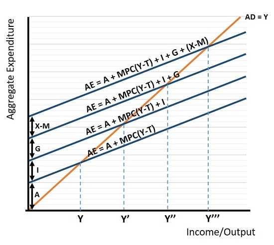
In the aggregate expenditure graph below, the lower blue line is the simple consumption function. The parallel lines above it represent the additions of the other three components of expenditure i.e., investment, government spending, and net exports.

Increases in autonomous consumption, investment, government spending, or net exports lead to parallel increases in aggregate expenditure.

The lines above the consumption function are drawn parallel to it because only consumption is considered to be an endogenous component i.e. directly influenced by income. Investment, government spending, and net exports are all exogenous.

In fact, even consumption has an exogenous part i.e., autonomous consumption. Autonomous consumption is exogenous because it represents that amount of consumption that is necessary even when income is zero. It is funded by borrowing, not income.

As with the consumption function, the slope of the basic aggregate expenditure model is determined by the marginal propensity to consume. When consumers increase the rate of spending, and thereby reduce their rate of saving, the slope of the aggregate expenditure function will get steeper and the multiplier effect will be greater (see below for details).

Equilibrium in the Aggregate Expenditure Model

Equilibrium in the model occurs when aggregate expenditure equals aggregate output i.e., where aggregate expenditure intersects the AD = Y line in the graph. This means that the level of aggregate demand (or planned aggregate expenditure) in the economy is in balance with the level of income/output.

When aggregate expenditure exceeds aggregate output, there is an unplanned decrease in inventory investment, which prompts businesses to increase production. On the other hand, when aggregate expenditure falls short of aggregate output, there is an unplanned increase in inventories, leading businesses to reduce production. In either case the economy will gravitate back towards equilibrium.

Achieving equilibrium is crucial for maintaining a stable economy and avoiding inflation or recession. Through analyzing the components of the aggregate expenditure model, Keynesian economists try to identify the factors that drive changes in aggregate expenditure so that they can guide policymakers in promoting equilibrium faster than would occur naturally.

The Four Components of the Aggregate Expenditure Model

The Aggregate Expenditure Model is a macroeconomic model that helps us understand the determinants of aggregate demand in an economy. It is based on the idea that total spending in an economy determines the level of output and income. Let's take a closer look at the key components of the model:

• The consumption function represents the relationship between disposable income and consumer spending. It shows how changes in income impact consumption behavior. In simple terms, as income increases, people tend to spend more.
• Investment spending refers to spending by businesses on capital goods, such as machinery, equipment, and buildings. The investment function captures the relationship between the level of investment and factors such as interest rates, business confidence, and technological advancements. Changes in these factors can significantly impact investment decisions.
• Government spending (fiscal spending) includes expenditures on goods and services, such as defense, education, healthcare, and infrastructure. Discretionary fiscal policy is a powerful tool for policymakers to stimulate or stabilize the economy.
• Net exports represent the difference between a country's exports and imports. They are influenced by factors such as exchange rates, trade policies, and global economic conditions. When a country's exports exceed its imports, it has a trade surplus, contributing positively to aggregate demand. Conversely, a trade deficit, where imports surpass exports, has a negative impact on aggregate demand.

The Multiplier Effect

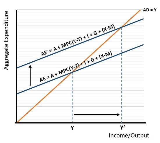
The Keynesian multiplier effect is a key concept in the Aggregate Expenditure Model just as it is in the consumption function. It explains how changes in spending can have a magnified impact on the overall level of output and income in an economy. This is illustrated in the graph below by the larger impacts on output resulting from a shift in aggregate expenditure.

A small upward shift in Aggregate Expenditure leads to a multiplied increase in Income/Output.

The multiplier effect occurs because an initial increase in spending leads to an increase in income, which, in turn, leads to additional spending. This process continues, causing a ripple effect throughout the economy.

The size of the multiplier depends on the marginal propensity to consume (MPC), which represents the proportion of additional income that is spent. The higher the MPC, the steeper the AE function and the larger the multiplier will be.

Criticisms and Limitations

While the Aggregate Expenditure Model forms a central role in mainstream economics and government policy making, it also has its limitations and has faced fierce criticism from competing economic schools of thought.

One criticism is that it assumes a constant marginal propensity to consume and a linear relationship between income and consumption. In reality, these relationships can be much more complex, and subject to volatility.

Additionally, being a Keynesian model, it assumes that prices are fixed in the short run. This does not always hold true. Furthermore, even when prices are stable, the model does not account for factors such as income distribution, wealth inequality, and expectations. These can all significantly impact consumer spending and investment decisions.

Finally, a critical limitation of the model relates to the incomplete modelling of consumption. Keynes’ fundamental psychological law simply states that consumption rises as income rises, but at a slower rate. That being the case, the other influences on consumption such as wealth, credit spending, and expectations, while not missing from the model, are treated as external to the model.

More advanced versions of the model do try to account for interest rates with respect to their influence on investment spending and consumption. Keynes’ liquidity preference theory describes the various sources of demand for money, but that theory is itself controversial.

All this points to the simple fact that any real-world attempt at modeling such complexities is verging on impossible. Added to this complexity is the difficulty of accounting for various policy lags that arise with any active attempt at demand-management.

In a nutshell, putting Keynesian theory to use in a reliable and effective way is practically impossible. Rather than leaving it to state planners to intervene in the economy as they see fit, there is a very strong case for leaving it market forces to self-correct any disequilibrium that occurs.

Conclusion

In conclusion, the Aggregate Expenditure Model is a fundamental concept in Keynesian economic thinking that attempts to understand the interactions between consumption, investment, government spending, and net exports.

By analyzing the key components of the model, such as the consumption function, investment spending, government spending, and net exports, these economists try to gain insights into the determinants of aggregate demand that can guide policymakers in making informed decisions.

While the aggregate expenditure model has its limitations, it remains a mainstream tool for analyzing the state of the economy, designing economic policies, and informing business decisions. How long this remains the case given the global debt levels that have accumulated in recent decades is anyone’s guess, but something big has got to change because the current mainstream approach to economics is not sustainable.

Sources:

• Romer, C. & Romer, D. - Planned Aggregate Expenditure and Output (PDF)

Related Pages:

• How do lower taxes affect aggregate demand
• How to calculate aggregate demand
• How does government spending affect aggregate demand

ShareFacebookXPinterestTumblrRedditWhatsApp