The Expansion Path in Economics

In economics, the expansion path is a concept that relates to the growth of a firm, and how it increases its production inputs in order to create more output. It does this by keeping its costs of production at their lowest points for any given level of output.

In order to understand the expansion path, it is necessary to first understand the constituent parts that are used to build the concept. Namely, these are:

• The Isoquant Curve
• The Isocost Line

Click the links for details, and to see how these two dynamics interact, have a read of my article about Cost Minimization. The expansion path is basically a long run model in which the firm under scrutiny is able to increase its desired capital and labor combinations in order to expand production efficiently. The graph below illustrates this.

Long Run Expansion Path Graph

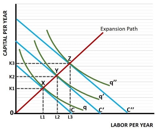
The long-run expansion path is illustrated by the red line, in the graph below, that passes through the origin. For this to be an accurate representation of the true long-run expansion path, we assume that the firm is operating in a competitive industry and is a price taker regarding its input costs.

We also assume, for simplicity, that there are no economies of scale in the production process. This means that any increase in output is matched by a proportionate increase in costs i.e., if it costs $100 to efficiently produce 50 units of output, then it will cost $200 to produce 100 units efficiently, and $300 to produce 150 units efficiently, and so on.

How do you calculate the expansion path?

The expansion path of the firm is given by connecting all the points of tangency between all relevant isoquant curves and isocost curves. These are illustrated in the long-run expansion path graph above at points X, Y, and Z. Drawing a straight line through these points and through the origin gives us the expansion path, as illustrated by the red line.

The expansion path shows us the efficient combinations of labor and capital i.e., those that minimize costs at various output levels.

The Long-Run Total Cost Curve

In this simple model we can calculate the firm’s long-run total cost curve if we know the cost of a unit of labor and a unit of capital. Remember that we assume the firm is operating in a competitive market and is a price taker with regard to input costs.

Under these conditions, the long-run total cost curve will be a straight line that slopes upwards and passes through the origin, just like the expansion path. All we need to do is multiply each of the two inputs, labor and capital, by their unit costs and add them together.

The Short-Run Expansion Path

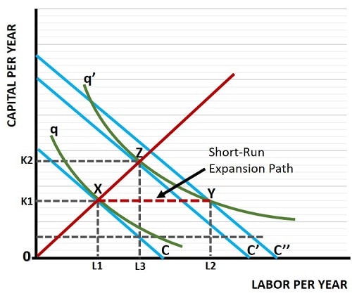
As always in economics, the short-run refers to the time period where only labor is a variable input, capital is fixed input. Clearly this has implications for the firm’s expansion path in the short-run, and in the graph above I have illustrated how this plays out.

Starting at point X, with L1 labor inputs and K1 capital inputs, the firm decides that it would like to increase production. The original output is illustrated by the isoquant curve q, but the firm wants to produce q’. In the long-run the efficient cost minimizing combination of inputs would be L3 and K2. However, with capital fixed at K1, the short-run expansion path follows the horizontal dashed red line as shown.

With L2 and K1 inputs, the firm can produce q’ output, but this occurs at the intersection of q’ and C’’ at point Y. Clearly, this is a higher isocost line than the long-run efficient isocost curve C’, meaning that the short-run expansion path incurs extra costs until capital can be increased. Until that time, the firm must use a lot more labor to compensate for the lack of capital, as illustrated by point Y. In the long-run, as capital is increased, labor will be reduced, as shown at point Z where L3, K2 is the cost minimizing point.

Expansion Path Formula

The expansion path formula relates to the Marginal Rate of Technical Substitution (MRTS) when a firm is operating efficiently at minimum cost i.e., where the following condition is being satisfied:

MPL/MPK = w/r

For more information on this, see my article about the MRTS.

Summary & Final Thoughts

The expansion path in economics refers to the trajectory of a firm's production and output as it increases its scale of operations. This concept is often associated with the long-run production function, where all inputs can be varied.

It typically demonstrates how a firm optimally adjusts its input combination to maximize output while minimizing costs as it expands its production scale. The concept is influenced by factors such as technology, input prices, and economies of scale, providing insights into a firm's long-term production strategies.

The simplified version above resulted in a linear expansion path, but in non-competitive industries where input prices can be negotiated by big firms, this will not be the case. Similarly, if there are economies of scale (or diseconomies) the curve will not be linear. Finally, if technology changes then this will affect the marginal product of capital which will, in turn, affect the cost minimizing expansion path.

Some potential controversies or points of discussion may include:

• Assumptions about Input Flexibility - In reality, some inputs may have constraints or face limitations in terms of availability or adjustability, and this can impact the accuracy of the model discussed above, which simply assumes complete input flexibility.
• Social Considerations - Critics might argue that the expansion path concept doesn't adequately account for externalities, sustainability, or social impacts. As businesses expand, there could be concerns about resource depletion, environmental degradation, or social consequences.
• Behavioral Considerations - Rational decision-making by firms is assumed. However, in reality, firms may not always behave in a strictly rational manner, and various market failures like moral hazard, adverse selection, the principal-agent problem, and so on may come into play.

These controversies highlight that while the expansion path is a valuable theoretical tool, its application and interpretation need to be considered in the context of specific real-world scenarios.

Related Pages:

• Productive Efficiency
• Costs of Production
• The Production Possibilities Curve

ShareFacebookTwitterPinterestTumblrRedditWhatsApp