Cost Minimization Analysis, Formula & Graphs

Cost minimization analysis, in microeconomics, is focused on finding the most efficient combination of inputs that a firm can use to produce a given output. By ‘inputs’ we mean all the resources that are used to create goods and services. Profit maximization and cost minimization go hand-in-hand, and we also assume that firms desire both.

Since we are looking at how to minimize the cost of those inputs, it stands to reason that we are assuming that firms can adjust the amounts used. The point here is that we are focusing on the long-run. Short-run microeconomic models hold capital is fixed and only labor as a variable input.

My article about productive efficiency refers to cost minimization in the context of the entire economy, where all goods and services are produced at the lowest cost. In this article I will focus on efficiency at the level of the firm, rather than the entire economy, and on the production of a given amount of output for one particular good.

Cost Minimization Graphs

The cost minimization graph below uses two concepts that I have discussed in separate articles. To understand the analysis here you will need to understand these concepts first, don’t worry, they are quite simple. For details, see:

• The Isocost Line
• The Isoquant Curve

In the graphs below, we simplify the cost minimization analysis by restricting the inputs under inspection to capital and labor. More complicated models do exist that use a more comprehensive array of inputs, but it is not possible to illustrate these with 2-dimensional graphs.

Restricting the analysis of cost minimization to labor and capital is standard practice in undergraduate microeconomics, because it helps us to grasp the basic concepts.

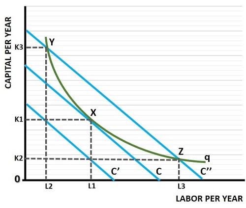
In the cost minimization graph above, capital and labor inputs are illustrated on the vertical and horizontal axes respectively. These costs should be considered on a units-per-year basis. We also assume that the firm under inspection is operating in a competitive market and that, consequently, it has no market power to influence the prices of capital or labor.

We take the price of labor as the wage rate (w) and the price of capital as the rental rate (r). We use the rental rate for simplicity, nothing fundamental changes if the firm purchases capital rather than rents it. See my article about the User Cost of Capital for more details.

Starting with the green isoquant curve (q) in the graph above, this curve plots all possible combinations of inputs that can be used to create a desired amount of output. The three blue isocost lines represent three alternative amounts of expenditure. Only isocost line C represents a cost minimization point, at point X in the graph.

Isocost line C’ does not intercept the isoquant at any point, which means that this low level of expenditure (costs) on inputs is insufficient to produce the desired output. Isocost line C’’ intercepts the isoquant curve at points Y and Z, meaning that the desired output can be produced with the input combination shown (L2, K3 and L3, K2 respectively) but the costs of doing so are higher than at point X.

Only where the isoquant curve just touches the lowest possible isocost line do we have a cost minimization point.

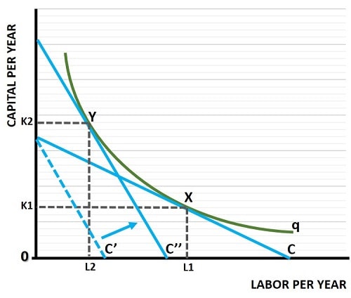
As explained in my article about the isocost line, the slope of the line depends on the relative prices of labor and capital i.e., its slope is equal to –(w/r). In the graph above, when the wage rate increases, the slope of the isocost line gets steeper, as illustrated.

Starting with isocost line C, the cost minimizing point is given at point X. However, if the wage rate were to rise relative to the rental cost of capital, a steeper Isocost line (the dashed line C’) will result. While this line still allows as much capital input to be used as before, but the higher cost of labor means that less can be used at the original expenditure/cost level.

In order to maintain production of the desired quantity of output, the firm must increase its costs until a new, steeper, isocost line just touches the isoquant curve. This is shown above by isocost C’’, which just touches the isoquant at point Y, the new cost minimization point.

Cost Minimization Formula

Intuitively we can understand that when costs are minimized, the relative amount of output gained from the last unit of labor must be equal to the relative amount of output gained from the last unit of capital, taking the costs of those inputs into account.

The cost minimization formula occurs where:

MPL/MPK = w/r

In words this can be stated as the cost minimization rule occurring where the marginal product of labor (MPL), divided by the marginal product of capital (MPK), is equal to the wage rate (w) divided by the rental cost of capital (r).

Cost Minimization Example

For example, imagine that one extra unit of labor costs $10, and that it can create 10 extra units of output. If the last unit of capital costs $40, then it must create 40 units of extra output. Any less than that would mean that the firm could reduce costs by using more labor units instead of capital units, and vice versa. For this reason, the cost minimization rule states that the formula above must be true.

Conclusion

Cost minimization analysis in economics is a strategic process employed by businesses and organizations to produce a desired level of output while keeping costs as low as possible. This involves a close examination of input costs, production technology, and the potential for input substitution.

Firms assess the costs associated with various inputs, primarily labor and capital, and study their relationship in order to identify the most cost-effective production methods.

Throughout this process, businesses aim to optimize resource utilization, enhance competitiveness, and maximize profits. The analysis extends to the production function, where the marginal and average productivities of inputs are studied to identify optimal combinations. It's about achieving efficiency and effectiveness in production by finding the right balance in input usage for a given level of output.

Related Pages:

• The Costs of Production
• The Expansion Path
• Marginal Rate of Technical Substitution MRTS
• Production Possibilities Curve

ShareFacebookXPinterestTumblrRedditWhatsApp