The Liquidity Trap Explained with Graphs

The liquidity trap is a situation that arises in economics when the money markets are unresponsive to the price of money i.e. interest rates. The possibility of such a situation arising had, until recently, been considered a theoretical abstraction with no historical examples in the real-world.

However, following the 2008 financial crisis, interest rates remained at historically very low levels for around 14 years, and the liquidity trap theory has received a lot more attention from economists since that time.

The theory itself was originally developed from the ideas of John Maynard Keynes and, regardless of whether it is a theoretical abstraction or a real-world phenomena, it does raise some interesting concepts that help to develop our general understanding of economics.

In the economic analysis that follows we use the simplifying assumptions that there is no significant inflation in the economy, and therefore the nominal interest rate is equal to the real interest rate.

The Liquidity Trap & IS-LM Graph Analysis

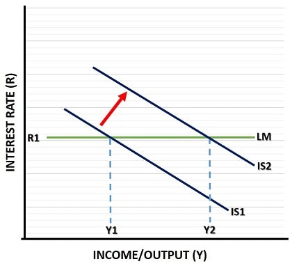
Using the basic IS-LM model to illustrate matters we can see that, in a liquidity trap scenario, any fiscal stimulus policy in the economy (such as increased government spending or a tax cut) will have no effect on the interest rate.

In words, the fiscal stimulus will directly boost the economy and lead to a higher income/output level. For example, consider a new government funded infrastructure project to build a new bridge that will reduce commuter times for workers and improve access to new markets for consumers on either side of the bridge.

This project will not only lead to more commercial activity, it will also directly increase salaries for construction workers and provide extra revenues for the suppliers of the raw materials that went into building the bridge. As a result of this, a new IS curve emerges, shifting from IS1 to IS2 in the graph above, which represents the increased spending in the goods market.

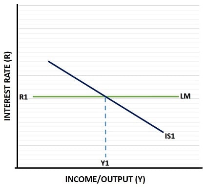
If Keynesian economic theory is correct, and there is spare capacity in the economy to sustain an increased level of income/output without raising the current price level, then the economy can grow from its original level of output at Y1 to Y2. This occurs at the new intersection of the IS2 curve with the LM curve in the graph.

So far this is all standard stuff.

However, the extra spending in the economy, and the higher income/output level, will lead to an increase in demand for money. This is because people will wish to hold more money in order to increase their purchasing power in the marketplace. The LM curve represents the money market, and in normal times any extra demand for more money (purchasing power) will lead to an increase in the price of money, i.e. an increase in the interest rate.

This is where the liquidity trap comes in, because a normal LM curve should be upward-sloping representing a higher cost of money as demand for it increases, but in a liquidity trap the LM curve is horizontal. The upshot is that, regardless of the extra demand for money to increase purchasing power, the interest rate is not affected.

The question is why, and what circumstances might cause this to happen? Before moving on to that question, let's briefly turn away from the liquidity trap implications for fiscal policy, and have a look instead at the implications for monetary policy.

Monetary Policy Economics under the Liquidity Trap

Notice in the diagram that, with a horizontal LM curve, monetary policy (rather than fiscal policy) is totally useless. Any attempt by the Federal Reserve Bank to boost the money-supply with lower interest rates (i.e. shifting the LM curve to the right to a new intercept point with the IS curve) is impossible.

This situation can arise only in times when the interest rate is already at or near to zero, because at any other time the central bank can always cut its base rate (called the 'Federal Funds Rate' in the US) if it chooses to do so.

However, when the rate is already as low as it can go, shifting a horizontal curve to the right will always intercept the IS curve at the same point, with the same income/output level, and the same interest rate.

What could cause a Liquidity Trap?

There are two main economic scenarios in which a liquidity trap may present itself:

The Effects of Quantitative Easing i.e. Money Printing

A significant quantitative easing policy can create a situation in which a liquidity trap might appear, and indeed it seems as though one did appear throughout the western world in the years after the 2008-09 global financial crisis. The problem is twofold:

1. Interest rates are already so low that there is little capacity to reduce them further in any significant way, which means it's difficult to fuel extra demand for money/loans simply by making it cheaper to borrow.
2. Whilst the central bank can increase the monetary base with 'money-printing' tactics, significant monetary expansion usually requires that the high-street banks play along and increase their rate of lending.

With low interest rates (and therefore low profitability from lending) and a banking system that was struggling with solvency issues after making so many bad loans in the run up to the 2008 economic meltdown, the high-street banks had been reluctant to make any more risky loans.

Instead they preferred to invest in financial securities - which is the primary reason why so many stocks/equities became so expensive even while an emerging pandemic led the political elites to lockdown the global economy. Price to earnings ratios on the stock market rose to historical highs.

Of course, the inflated stock market following numerous rounds of quantitative easing was probably working just to delay an eventual burst of inflation rather than prevent it. In that case it would be incorrect to regard quantitative easing as a cause of a permanent liquidity trap, because once the extra money reaches the real economy and is spent in the goods market rather than the financial assets market, inflation should rise sharply, and interest rates too (as indeed happened in 2022).

A falling price level

Another historically rare situation occurs when the economy goes through a severe economic slowdown. In these circumstances a lack of spending in the economy can cause prices to start falling i.e. deflation.

When there is a significant amount of deflation in the economy, the value of cash increases over time, and that may encourage people to save it for later, rather than spend it today. This, of course, renders monetary policy ineffective since boosting the money-supply does not motivate people to go out and spend it.

Clearly, in times of low interest rates and an economic slowdown, this problem is more likely to present itself since the possibility of deflation is higher, and it is relatively cheap to hold onto money.

Here again, in a situation where massive amounts of money has been pumped into the system to keep the economy from going into a depression (i.e. current times), any prospect of deflation may be short-lived and quickly followed by sharp increases in inflation once the money that economic agents are holding onto starts being spent.

As with the quantitative easing scenario, the liquidity trap here may just be a temporary phenomena before reality blows the lid off of interest rates and inflation, with resulting economic chaos.

The Classical Case Explained (opposite of liquidity trap)

It seems customary, when presenting information about one extreme case in the Keynesian IS-LM framework, to also present the opposite extreme - i.e. the Classical Case.

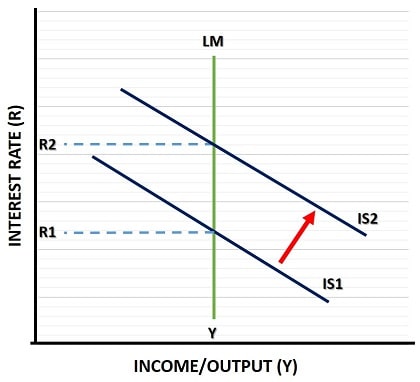
The classical case occurs when the economy is running at full capacity, meaning that any policy to boost the economy, whether it be fiscal or monetary, will fail and simply cause higher prices that offset the boost. In this scenario the LM curve is vertical as shown in the graph below, and fiscal policy expansion fails to increase income/output beyond its starting level of Y.

Alternatively, any monetary policy boost would fail to shift the LM curve because rising prices would erode the purchasing power of the boost, and thereby return the LM curve to its starting position (see my article about the LM curve for an explanation of this).

In reality, empirical evidence suggests that short-run economic boosts are entirely possible, but the 'rational expectations' school argues that even short-run effects will gradually become impossible as economic agents improve their expectations and reactions in the face of such policies from the government.

The rational expectations hypothesis gained a lot of support from some economic thinkers when it first appeared in the 1960s. Unfortunately, the news on that front is not encouraging, and I find little evidence of any increase in rational behavior from people when it comes to economics in modern times, but we live in hope.

Sources:

• Inflation and Liquidity Trap

Related Pages:

• The Money Multiplier
• The IS-LM Model
• The Monetary Transmission Mechanism
• Does Quantitative Easing Cause Inflation?

ShareFacebookXPinterestTumblrRedditWhatsApp