- Home
- Perfect Competition
- Deadweight Loss

Deadweight Loss Explained (Graph, Formula & Examples)
Deadweight loss, in economics, describes the loss of total economic welfare when a market is not operating at peak efficiency. In a perfectly competitive market, prices and quantities adjust so that the combined benefits to consumers and producers, known as total surplus, are maximized. When something disrupts this balance, such as a tax, subsidy, price control, or market power, the total surplus shrinks.
The portion of potential economic value that disappears entirely, rather than simply shifting from one group to another, is what economists call deadweight loss. At its core, deadweight loss arises when the quantity of goods traded falls short of the socially optimal level. This often happens because distortions raise prices for buyers or lower returns for sellers, causing fewer transactions to take place.
In this article I assume the standard market structures where there are no significant external market failures, this is true of most real-world markets but readers are encouraged to read further – my article about externalities (and related pages) will help with that. In the absence of externalities, taxes and other policies tend to reduce the total number of mutually beneficial trades, leading to a net loss of total surplus i.e., a deadweight loss.
Understanding deadweight loss is important for evaluating the real costs of policy decisions, market structures, and regulations – not just in terms of who gains or loses, but also in terms of the economic value that is lost to society as a whole.
Economic
Efficiency and Optimal Total Surplus
Economic efficiency occurs when the optimal allocation of resources to maximize the well-being of individuals and society as a whole is achieved. This concept is grounded in the idea that resources are scarce, and their optimal use is crucial for achieving maximum output and satisfaction.
To grasp the significance of economic efficiency, consider the example of a market for goods and services. In a perfectly competitive market, the forces of supply and demand interact to determine the market equilibrium price and quantity, this is illustrated in the graph below with price and quantity of p, q where optimal total surplus occurs.
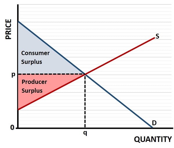 At a competitive market equilibrium, the supply and demand curves intersect at the price and quantity that maximize total surplus — demonstrating allocative efficiency before any distortions occur.
At the equilibrium point where demand intersects supply, the quantity of goods supplied matches the quantity demanded, ensuring that resources are allocated in the most productive way. Consumer surplus and producer surplus are simultaneously optimized, and the market operates without any waste. For more details about the two types of surplus, see my articles about:
Deadweight loss arises when economic efficiency is not achieved, and there are many factors that can cause this.
Causes of
Deadweight Loss
The causes of deadweight loss can be categorized into three main groups, these are price controls, taxes & subsidies, and monopoly power:
- Price Controls – Price ceilings, which set a maximum allowable price for a good or service, can lead to deadweight loss via shortages, because any artificially low price increases demand while discouraging supply. Conversely, price floors, which set a minimum price, can result in surpluses as the high price encourages more production while reducing demand. Both scenarios lead to an inefficient allocation of resources and a deadweight loss, as the market is unable to reach its natural equilibrium.
- Taxes & Subsidies – When taxes are imposed on goods or services, they create a difference between what consumers pay and what producers receive. This tax wedge distorts the market equilibrium, leading to reduced quantities traded and a loss of economic efficiency. Subsidies, while intended to promote certain economic activities, can also lead to deadweight loss by artificially lowering the price of a good or service leading to overproduction and overconsumption.
- Monopoly power – Where a single firm dominates a market, this can also lead to significant deadweight loss. In a monopolistic market, the monopolist has the ability to set prices above the competitive level, reducing the quantity of goods traded. This price-setting power leads to an allocation of resources that is not socially optimal, resulting in a deadweight loss.
Price
Controls and Their Role in Deadweight Loss
Price controls, such as price ceilings and price floors, are another form of government intervention that can lead to a potential deadweight loss. These controls are often implemented with the intention of protecting consumers or producers, but they can have unintended consequences that distort market efficiency. Price ceilings, for example, set a maximum allowable price for a good or service. While this may seem beneficial to consumers, it can lead to shortages as the artificially low price increases demand while discouraging supply.
An example of a price ceiling is rent control, where the government limits the amount landlords can charge for housing. While this policy aims to make housing more affordable, it can lead to a shortage of available rental units. Landlords may be less inclined to rent out properties at the capped price, and new construction may be discouraged.
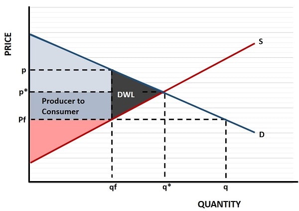 Deadweight loss arising from a price ceiling set below the market equilibrium: the quantity demanded exceeds supply, creating excess demand and lost total surplus.
The price ceiling graph above illustrates that a fixed price (Pf) set below the equilibrium price (p*) results in a market with excess demand for rental units, i.e. where (q) exceeds the quantity supplied (qf), leading to a deadweight loss (DWL) of surplus that neither consumers nor producers can capture. Producers, landlords in this example, are particularly hard hit because some of their previous surplus is given to consumers i.e. the remaining tenants who still have rental accommodation. This transfer of surplus is shown by the darker blue area in the graph.
Price floors, on the other hand, set a minimum allowable price for a good or service. An example is the minimum wage, which sets the lowest legal wage that employers can pay their workers. While the intention is to ensure a living wage for workers, a high minimum wage can lead to unemployment if employers cannot afford to hire as many workers at the mandated wage. The resulting surplus of labor supply, where the quantity of labor supplied exceeds the quantity demanded, leads to a deadweight loss, as illustrated in the graph below.
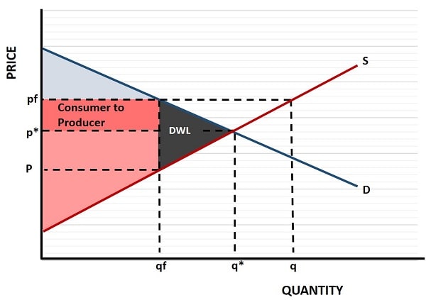 When a price floor such as a minimum wage is set above the equilibrium wage, the resulting excess supply of labor and reduced employment create a deadweight loss due to market distortion.
With a fixed price (Pf) set above the equilibrium price (p*), the quantity of workers wishing to supply their labor rises above the equilibrium level (q*) to q. However, employers are unable to profitably employ the extra workers at the higher wage, or even the pre-existing workers. The quantity of employed workers therefore falls to qf.
Those workers who retain their jobs benefit from the minimum wage at the expense of their employers, but the deadweight loss (DWL) occurs because some workers lose their jobs altogether, with no transfer of surplus and just a loss of overall surplus.
The Impact
of Taxes on Deadweight Loss
Taxes are a common tool used by governments to generate revenue, but they can also create significant deadweight loss. When a tax is imposed on a good or service, it raises the price that consumers pay but producers receive a lower price. This tax wedge reduces the quantity of the good traded, leading to a loss of both consumer surplus and producer surplus. This is illustrated in the graph below.
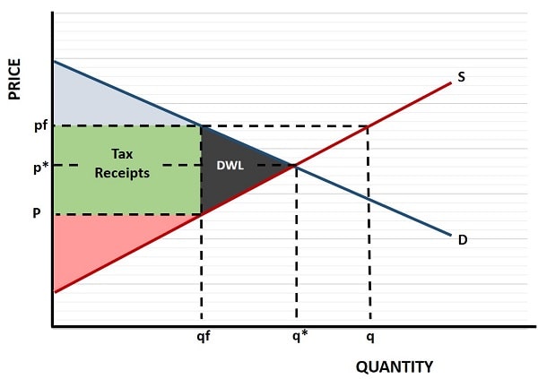 When a tax is imposed, the wedge between what buyers pay and what sellers receive reduces the traded quantity — the shaded triangle between the supply and demand curves represents the deadweight loss of economic efficiency.
With a tax set at pf – p, tax revenue is equal to the green area illustrated in the graph. The same deadweight loss occurs as with a price floor (described above), but in this case the transfer of surplus comes from both consumers and producers in favor of the government.
The extent of the deadweight loss depends on the price elasticity of supply and the price elasticity of demand. Elasticity measures how responsive consumers and producers are to changes in price. When demand is highly elastic, consumers reduce their quantity demanded significantly in response to a price increase caused by a tax. Similarly, if supply is elastic, producers reduce their quantity supplied.
In both cases, the reduction in quantity traded is large when elasticity is high, leading to a substantial deadweight loss. Conversely, if supply and demand are inelastic, the reduction in quantity traded is smaller, resulting in a smaller deadweight loss.
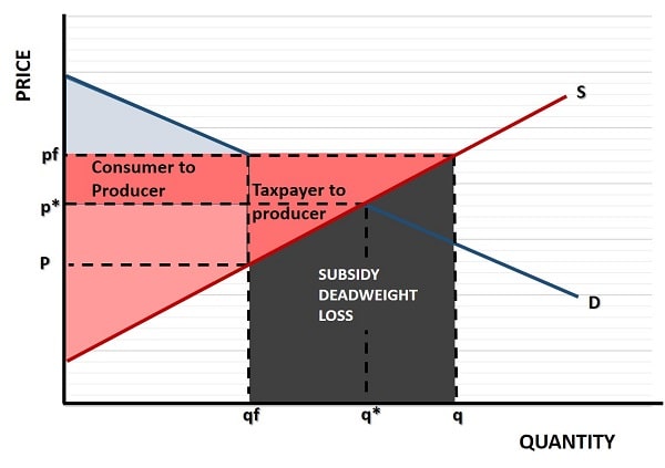 Subsidies that set prices above the market equilibrium can lead to overproduction and excess supply — the shaded area in this graph highlights the deadweight loss when resources are used inefficiently.
In the graph above I have illustrated what happens with a particularly poorly constructed subsidy policy. If the government promises farmers that they will buy up all of the wheat produce that they can’t sell at a fixed price of pf, which is higher than the market clearing equilibrium price of p*, those farmers will increase their production of wheat beyond the market clearing equilibrium output of q*, all the way to q. This creates an excess supply of wheat equal to q – qf, and the government will buy it at a price of pf. This costs the taxpayer pf(q – qf), and while some of this expense is transferred to farmers most of it is a deadweight loss in the form of a mountain of wheat that will go to waste.
Monopoly
Power and Deadweight Loss
In a perfectly competitive market, firms are price takers, meaning they accept the market price determined by supply and demand. The equilibrium price ensures that the quantity supplied matches the quantity demanded, maximizing total surplus. However, a monopolist, as the sole supplier, can restrict output to raise prices. This results in higher prices for consumers and lower quantities traded, leading to a loss of consumer surplus and an overall welfare loss to society.
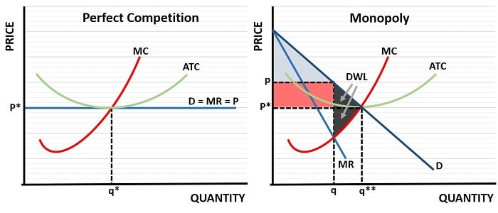 A monopoly restricts output and raises price relative to the competitive equilibrium, reducing traded quantity and creating a deadweight loss — shown here as the welfare triangle between monopoly and competitive outcomes.
Consider the graph above which illustrates an example of a pharmaceutical company with a patent on a life-saving drug. The patent grants the company monopoly power, allowing it to set high prices that many consumers may not be able to afford.
In perfect competition, each individual firm would sell the drug at a price of p* as illustrated on the left-side of the graph. Total market supply would be q** as indicted on the right-side of the graph. However, with a patent, the monopoly firm will reduce market supply to q, and charge a higher price of p. This results in a similar deadweight loss as would occur with a price floor (explained above) with a similar transfer of surplus from consumers to the monopolist. For explanations of the models illustrated in the graph, see my articles about:
Monopoly power can arise from various sources, including patents, control of essential resources, and government regulations. We should not automatically assume that any given monopoly is bad for society in the long run, even though they come with some potential deadweight loss.
In the example above, producing new drugs is a very expensive business with huge amounts of money spent on research and development. Pharmaceutical companies may be deterred from making these expensive new drugs unless they can recoup those costs via the profits that come with a patent. There are other examples where monopoly is the best option, but in general it is a sub-optimal market structure because of the inherent deadweight loss that occurs.
Real-World
Examples of Deadweight Loss
Real-world examples of deadweight loss can be found in various markets and policy interventions. I’ll reiterate the examples mentioned above, and add tariff policies as another deadweight loss generating example:
- Agricultural Subsidies – While these subsidies aim to stabilize farm incomes and ensure food security, they can lead to overproduction of certain crops. The excess supply, coupled with the cost of subsidies borne by taxpayers, results in a deadweight loss as resources are not used in their most valuable capacity.
- Rent control policies - These provide a clear example of deadweight loss in the housing market. By capping rental prices, these policies lead to a shortage of available housing units, and poor maintenance of remaining properties because landlords can easily replace existing tenants given the resulting excess demand.
- Tariffs & Import Quotas – Tariffs and quotas are intended to protect domestic industries by making foreign goods more expensive. However, they can lead to inefficiencies by reducing the quantity of goods traded and increasing prices for consumers, which causes a deadweight loss.
Deadweight
Loss Formula: Tools and Techniques
Calculating deadweight loss involves quantifying the lost economic value resulting from market inefficiencies. Several tools and techniques are used by economists to estimate deadweight loss and assess the impact of various policies, but there is no specific formula.
When using linear demand and supply functions, area of deadweight loss illustrated in the graphs above can be calculated as the triangular area between the supply and demand curves, with the base of the triangle corresponding to the reduction in quantity traded and the height representing the price difference caused by the intervention.
Another approach involves the use of econometric models to analyze data and estimate the elasticity of supply and demand. By estimating elasticity, economists can predict how changes in taxes, subsidies, or price controls will affect market outcomes and the resulting deadweight loss.
Cost-benefit analysis is also a valuable tool for measuring deadweight loss. This technique involves comparing the costs and benefits of a particular policy or intervention to assess its overall impact on economic welfare.
Policy
Implications and Solutions to Minimize Deadweight Loss
I mentioned in the introduction to this article that I was assuming a lack of any significant external market failures, and this is important because where such externalities do exist there may be opportunities to actually increase societal welfare by use of various Pigouvian subsidies and corrective taxes to achieve a socially optimum quantity and price.
For example, rather than imposing broad-based taxes that affect the entire economy, policymakers can implement targeted taxes on goods with negative externalities, such as pollution. By taxing activities that generate external costs, the government can correct the market failure without creating significant deadweight loss. Similarly, subsidies can be designed to support essential services or promote positive externalities, such as education and healthcare, without encouraging overproduction or overconsumption.
Another solution is to implement flexible price controls that allow for market adjustments. For instance, rather than setting rigid price ceilings or floors, policymakers can use sliding scales or indexed prices that adjust based on market conditions. This approach helps prevent the extreme shortages or surpluses associated with fixed price controls, reducing the deadweight loss.
Antitrust laws and regulations that prevent the abuse of market power can help ensure that markets remain competitive and efficient. By fostering a competitive environment, policymakers can reduce the deadweight loss associated with monopoly power and promote more equitable economic outcomes.
Ultimately, the goal of economic policy should be to create a framework that allows markets to operate efficiently while addressing specific market failures and promoting social welfare.
FAQs
Why is deadweight
loss considered a measure of market inefficiency rather than just a transfer of
wealth?
Why is deadweight
loss considered a measure of market inefficiency rather than just a transfer of
wealth?
Because deadweight loss represents transactions that never occur, it reflects the loss of potential value to society as a whole. In contrast, a transfer of wealth simply moves value from one group to another without reducing total surplus.
Can deadweight loss
occur in labor markets without government intervention?
Can deadweight loss
occur in labor markets without government intervention?
Yes. For example, mismatches between workers’ skills and job requirements, or rigid hiring practices in monopolistic industries, can reduce the number of mutually beneficial employment contracts, creating deadweight loss.
How do international
trade restrictions contribute to deadweight loss?
How do international
trade restrictions contribute to deadweight loss?
Trade barriers such as quotas and tariffs prevent goods from being exchanged where they have the highest value, raising prices domestically and reducing consumption and production efficiency globally.
What role does time
play in the magnitude of deadweight loss?
What role does time
play in the magnitude of deadweight loss?
In the short term, supply and demand may be inelastic, making deadweight loss small. Over time, as producers and consumers adjust behavior, the quantity distortion can grow, increasing deadweight loss.
How can behavioral
economics explain consumer reactions that worsen deadweight loss?
How can behavioral
economics explain consumer reactions that worsen deadweight loss?
Cognitive biases such as loss aversion or anchoring can cause consumers to overreact to price changes from taxes or controls, leading to sharper drops in demand than classical models predict.
Can deadweight loss
occur in non-monetary economies?
Can deadweight loss
occur in non-monetary economies?
Yes. Even in barter or resource-based economies, restrictions, monopolies, or inefficiencies can prevent optimal trade, causing a loss in overall utility that parallels monetary deadweight loss.
Conclusion
Deadweight loss represents more than just a technical concept in economics – it is a practical measure of the costs society bears when markets fail to operate at peak efficiency. Whether caused by taxes, subsidies, price controls, or monopoly power, the result is the same: fewer mutually beneficial trades and a reduction in total surplus. While some market interventions are necessary to address externalities or achieve social goals, the challenge for policymakers lies in balancing these objectives with the need to preserve efficiency.
Related Pages:
- Profit Maximization
- Market Equilibrium
- Import Quotas vs Tariffs
- Perfect Competition
About the Author
Steve Bain is an economics writer and analyst with a BSc in Economics and experience in regional economic development for UK local government agencies. He explains economic theory and policy through clear, accessible writing informed by both academic training and real-world work.
Read Steve’s full bio
Recent Articles
-
What Happens to House Prices in a Recession?
Jan 11, 26 03:13 AM
What happens to house prices in a recession? Learn how different recessions affect housing, why 2008 was unique, and how policy responses change home values. -
Does Government Spending Cause Inflation?
Jan 10, 26 06:01 AM
Does government spending cause inflation? See how waste, crowding out, and stimulus spending quietly push prices higher over time. -
What Happens to Interest Rates During a Recession
Jan 08, 26 05:31 PM
What happens to interest rates during a recession? Explore why rates often fall, when they don’t, and how inflation, policy, and markets interact. -
Circular Flow Diagram in Economics: How Money Flows
Jan 03, 26 04:57 AM
See how money flows through the economy using the circular flow diagram, and how spending, saving, and policy shape real economic outcomes. -
What Happens to House Prices During Stagflation?
Jan 02, 26 09:39 AM
Discover how house prices and real estate behave during stagflation, with historical examples and key factors shaping the housing market.