The Budget Line & Budget Constraint

The budget line in economics is used in the standard two-good model to illustrate all affordable baskets of goods that a consumer can afford given his/her limited income. Whilst the real world may have a few billionaire exceptions, most of us do face a restrictive budget constraint that forces us to allocate our spending with care.

On this page I will continue with the standard assumptions of the basic consumer behavior model, meaning that a consumer's preferred baskets of goods are complete and transitive, and that more goods are always preferred to fewer goods. I have explained these assumptions in more detail on my main page about consumer behavior, so click the link if you need a refresh on that.

The budget line graph below illustrates the budget constraint faced by a consumer; it is represented by a straight line that touches both the vertical axis and the horizontal axis.

Slope of the Budget Line

In the budget line graph below, we show all combinations of the two goods biscuits and cheese that a consumer can afford. All points on the budget line infer that the consumer has allocated his/her entire income to purchasing some basket of these goods.

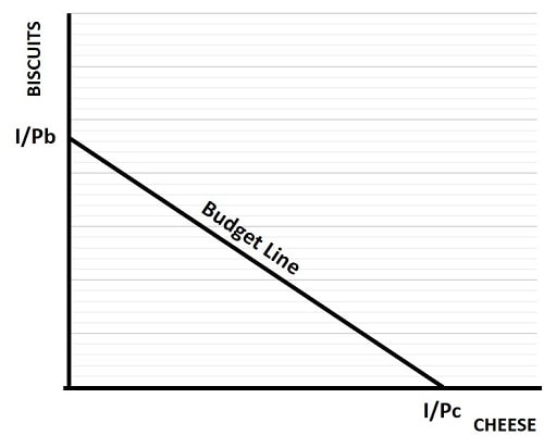
If the consumer were to spend all of his/her income on biscuits, then quantity of biscuits purchased would be equal to income divided by the price of biscuits. This is illustrated by the vertical quantity I/Pb. Similarly, if all of the income is spent on cheese, then I/Pc on the horizontal axis represents the quantity of cheese purchased.

When all income is spent on these goods, the budget line is given by the equation:

I = B(Pb) + C(Pc)

Since any individual consumer is regarded as a price-taker, we assume that the consumer is unable to negotiate a better price for either good regardless of what proportion of his/her income is allocated to purchasing it. With prices fixed, that gives us a straight budget line with a downward (or negative) slope equal to the ratio of the two prices.

Mathematically, the slope is equal to -1(I/Pb)/(I/Pc), which transposes to:

Budget Line Slope = -Pc/Pb

All consumption bundles that lie below the budget line are affordable, but they do not optimize utility for the consumer and are therefore regarded as suboptimal i.e. less preferred than at least one other possible bundle. All points above the line are unaffordable, and although they may be preferred this is not necessarily the case. Remember that it is the indifference curve that illustrates preferences, not the budget line, so we cannot use a budget line alone to determine all preference points.

The Budget Line and Indifference Curve

When a consumer chooses to optimize his/her utility, i.e. satisfaction level, he/she will be consuming a basket of goods that sits along the highest indifference curve possible given the budget constraint of limited income. Utility is optimized at the point that this indifference curve just touches the budget line, as illustrated in the graph below.

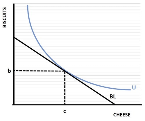
Only with quantities of b biscuits and c cheese is the utility maximizing basket of goods achieved. All other baskets are either suboptimal or unaffordable. Notice also, that when the indifference curve just touches the budget line, the budget line is tangential to the indifference curve. When this happens, the slope of the budget line is equal to the marginal rate of substitution (MRS) (click the link for details on that.)

The question arises as to whether or not the slope of the budget line is always equal to the MRS, and the answer is no. There are some relatively rare occasions known as 'corner solutions' where the slope is different, see below for details. 

The Budget Constraint given Limited Income

The budget constraint is representative of one of the founding principles in economics i.e., that of scarcity. I mentioned earlier that some people are billionaires, and clearly fortunate enough to have seemingly unlimited budget constraints. This may be true, but the problem of scarcity is not entirely overcome by more or less unlimited purchasing power. Even billionaires have other constraints to deal with - most notably time.

Consumption of one good may negate consumption of another once time is added to the picture e.g., we may like to purchase an all expenses paid trip to Milan, but we cannot simultaneously enjoy a trip to Madrid.

Constraints abound in the real world, but in economics we focus on primarily on the budget constraint and limited income, because it is the one constraint that best helps us to explain consumer behavior.

Budget Line Formula

A useful way to remember the budget line is to regard as the line that separates that which is affordable and that which is not. With this in mind it is easy to remember that all points on the line infer that all income is being spent. This can be represented in a formulaic expression that includes all goods consumed rather than being restricted to the two-good model above:

I = A(Pa) + B(Pb) + C(Pc) + D(Pd) ...

This simple formula just adds up all of the spending on individual goods in order to derive the budget line formula. There can be as many or as little goods included, but it becomes impossible to represent this in a graphs. Three goods would require a three dimensional plane rather than a two dimensional line, and I've no clue what a graph with more than three dimensions would look like.

Budget Line Example (changing prices & income)

In the examples below I've illustrated what happens to the budget line when the price of a good decreases, and when the disposable income of a consumer increases.

Consumer spending and price changes

With a price change, the effect leads to a pivot of the budget line around the point at which it touches one axis or the other. In the example below I've illustrated what happens when the price of good x on the horizontal axis decreases from x to x'. At the lower price, the consumer finds that a greater quantity of this good can be purchased (up to the limit I/Px').

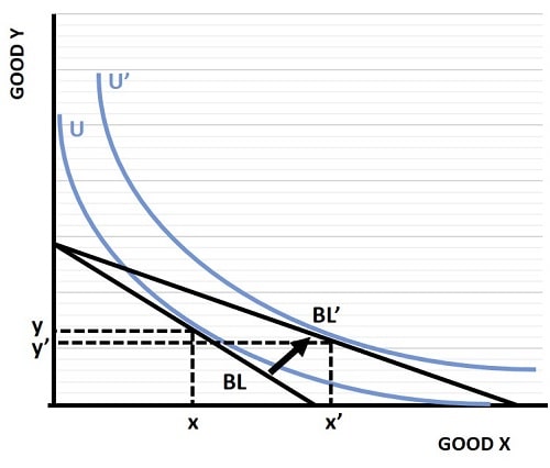
The effect of this is to pivot the budget line around its intersection point on the vertical axis to a new higher line (from BL to BL'). With a higher budget line, the consumer is able to afford baskets of goods on a higher indifference curve, and moves from a basket of x,y  to x'y'.

Notice here that the lower cost of good x has actually led the consumer to increase his/her consumption of it so much that consumption of good y is reduced compared to the original basket. This is not forced to happen, but it is certainly possible that such things can happen depending on the types of goods involved. For details on this, see my article about the price consumption curve.

Income changes shift the Budget Line

In the next example I've shown how an increase in income leads to a higher budget line at all points, not just a pivot around one good. If prices are help constant, the increase in income will lead to a higher budget line that is parallel to the original line, as illustrated by the shift from BL to BL' in the graph below.

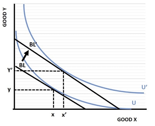
An increase in income will tend to lead to an increase in demand for both goods, as illustrated by the move from basket x,y on the lower indifference curve, to x'y' on the new higher indifference curve. Again, it is not guaranteed that demand for both goods will increase with higher income, it all depends on the types of goods under analysis. For details on this, see my article about the income consumption curve.

A Corner Solution

I mentioned above that there is a scenario in which the preferred basket of goods at the highest affordable indifference curve can, in extreme circumstances, occur where the MRS has a different slope to the budget line. One such scenario is illustrated below, it is called a corner solution.

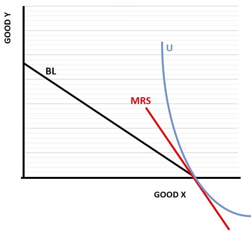
With a corner solution, the consumer's preference is to spend all of his/her income one good only, and would like to consume even more of that good if it were affordable. This leads to a situation in which the indifference curve passes through the highest achievable quantity of the preferred good, rather than just touching that point.

This happens in the graph above for good x, and the slope of the MRS line is greater than the slope of the budget line in this situation. If you recall that the slope of the budget line is given by -Px/Py, this corner solution arises where MRS > -Px/Py.

It is also possible that a corner solution could occur on the other axis, with an indifference curve that is flatter than the budget line. In that case MRS < -Px/Py.

Related Pages:

• Revealed Preference
• Intertemporal Budget Constraint
• Marginal Utility
• Consumer Behavior

ShareFacebookXPinterestTumblrRedditWhatsApp